CLASHub Analyzer Tutorial
This tutorial covers the five main analysis modules available in the Analyzer: CLASH, miRNA-seq, RNA-seq, cumulative fraction curve generation, and job status monitoring.
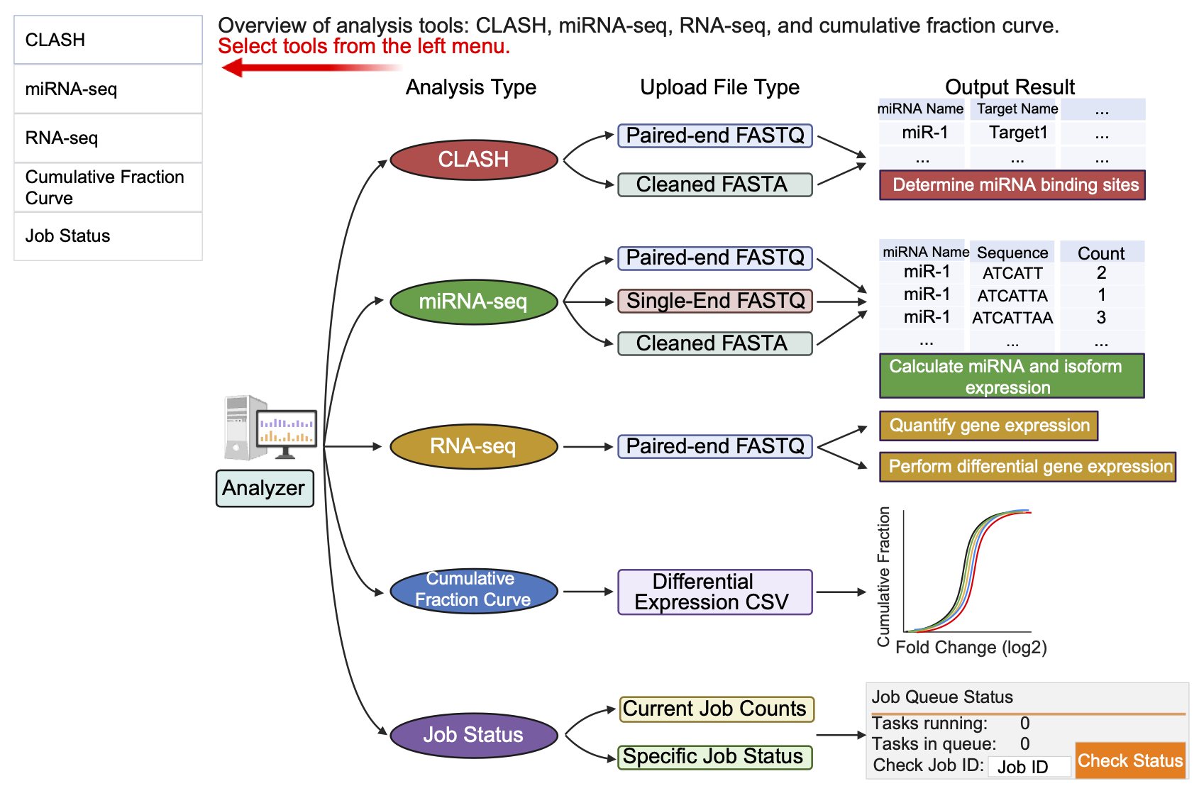
Schematic representation of the five main modules available in the CLASHub Analyzer interface, including CLASH (red), miRNA-seq (green), RNA-seq (orange), cumulative fraction curve generation (blue), and job status monitoring (purple). Users can select the desired analysis type from the left menu. Each module specifies compatible input file formats and outlines the corresponding output content.
CLASH analysis
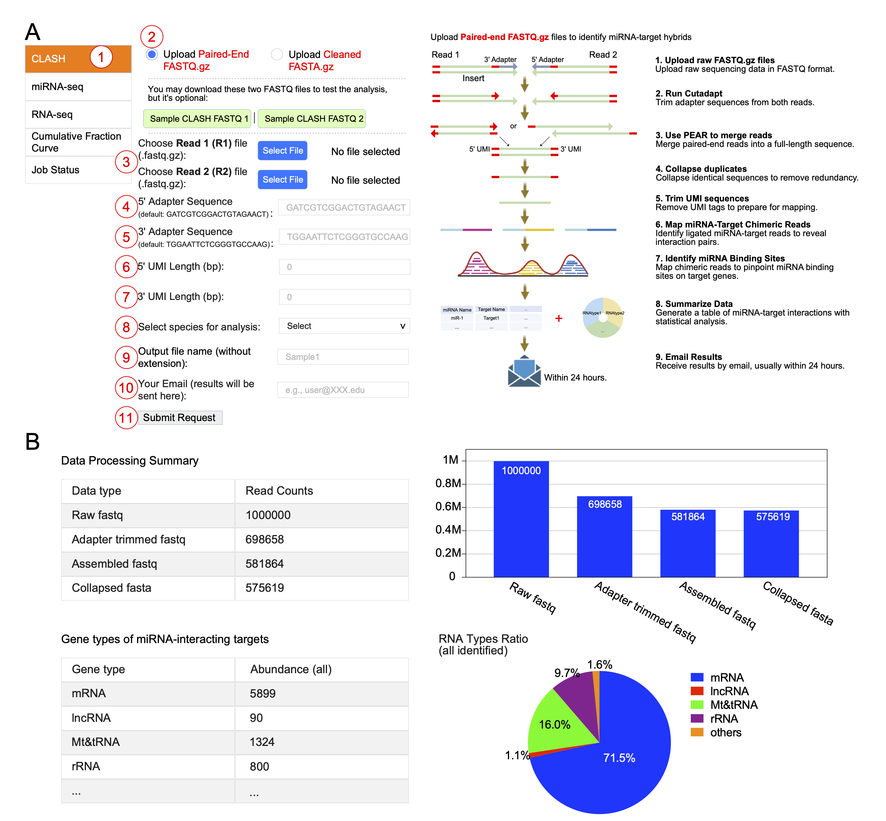
(A) Interface for initiating CLASH analysis. Users 1 select the CLASH module, 2 select input file type, 3 select local sequencing files for upload, 4 and 5 input adapter sequences, 6-7 define the length of 5′ and 3′ Unique Molecular Identifiers (UMIs), 8 select species, 9 specify output filename, and 10 enter email address, then 11 submit the request. The backend bioinformatic pipeline to process paired-end FASTQ data is shown on the right.
(B) Example output report, displaying processed read counts, RNA type summary, and RNA composition chart.
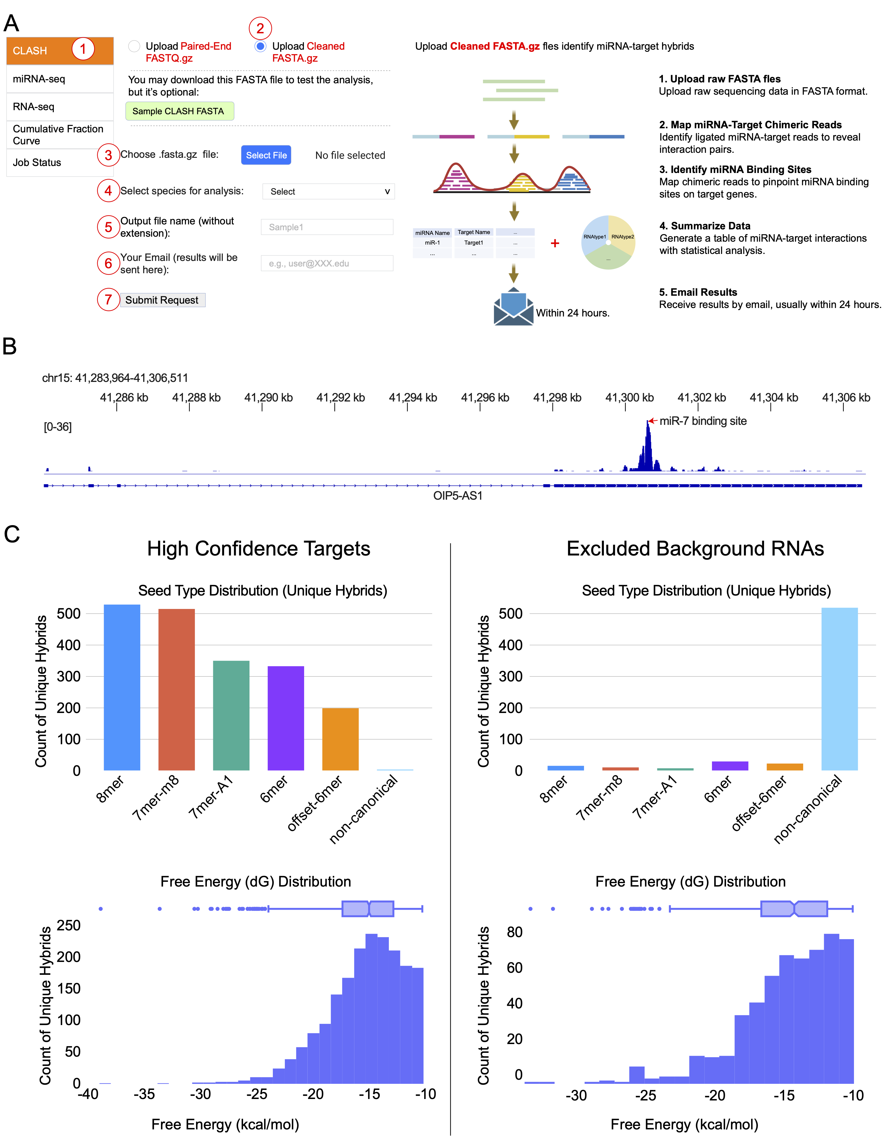
(A) Interface for submitting CLASH analysis with cleaned FASTA files. Users 1 select the CLASH module, 2 choose “cleaned FASTA.gz” as input file type, 3 select a local FASTA file for upload, 4 select species, 5 specify output filename, 6 enter email address, and 7 submit the request. The backend bioinformatic pipeline to process cleaned FASTA data is shown on the right.
(B) Genome-level visualization of CLASH-mapped reads. For each submitted FASTA file, CLASHub generates a bigWig (bw) file for inspection in IGV. Shown is an example of miR-7 binding to OIP5-AS1 (Cyrano) in the human hg38 genome.
(C) Example of the comparative quality assessment report generated by the CLASH analysis module. The charts visualize the characteristics of unique miRNA-target hybrids by distinguishing High Confidence Targets from Excluded Background RNAs (e.g., rRNAs, tRNAs, mitochondrial RNAs, and pseudogenes).
miRNA-seq analysis
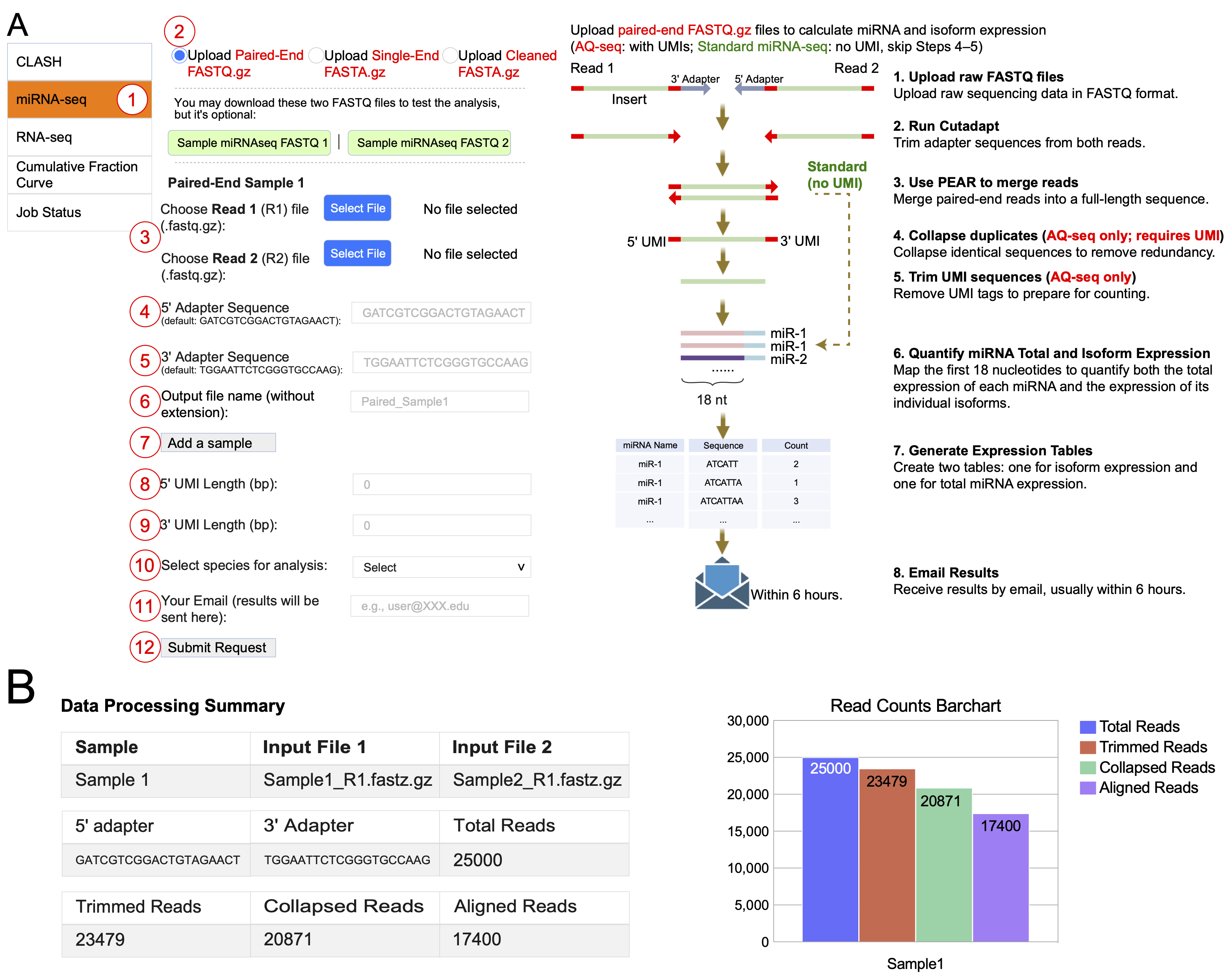
(A) Interface for miRNA-seq analysis. Users 1 select the module, 2 choose input file type, 3 select paired-end FASTQ files to upload, 4-5 enter adapter sequences, 6 specify output filename, 7 can optionally add additional samples, 8-9 define the length of 5′ and 3′ Unique Molecular Identifiers (UMIs), 10 select species, 11 provide email address, and 12 submit the request. The backend bioinformatic pipeline to process paired-end FASTQ data is shown on the right.
(B) Output summary and a bar chart displaying statistics of the processed reads.
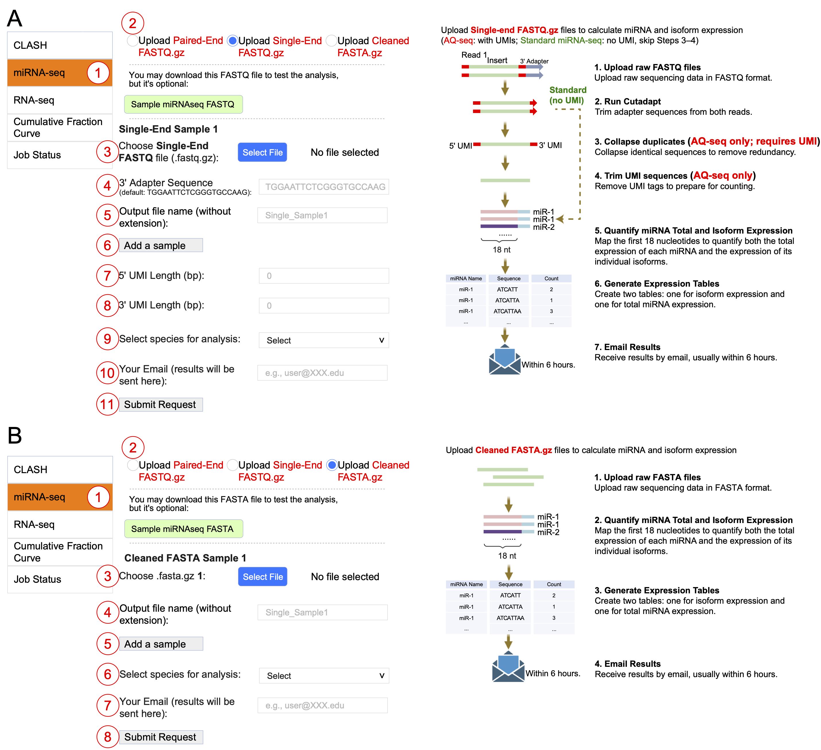
(A) Interface for processing single-end FASTQ files. Users 1 select the miRNA-seq module, 2 choose the “Single-End FASTQ” input, 3 choose a local file to upload, 4 enter the adapter sequence, 5 specify the output filename, 6 can optionally add additional samples, 7-8 define the length of 5′ and 3′ Unique Molecular Identifiers (UMIs), 9 select the species, 10 provide an email address, and 11 submit the request.
(B) Interface for processing cleaned FASTA files. Users 1 select the miRNA-seq module, 2 choose the “Cleaned FASTA” input, 3 choose a local file to upload, 4 specify the output filename, 5 can optionally add additional samples, 6 select the species, 7 provide an email address, and 8 submit.
RNA-seq analysis
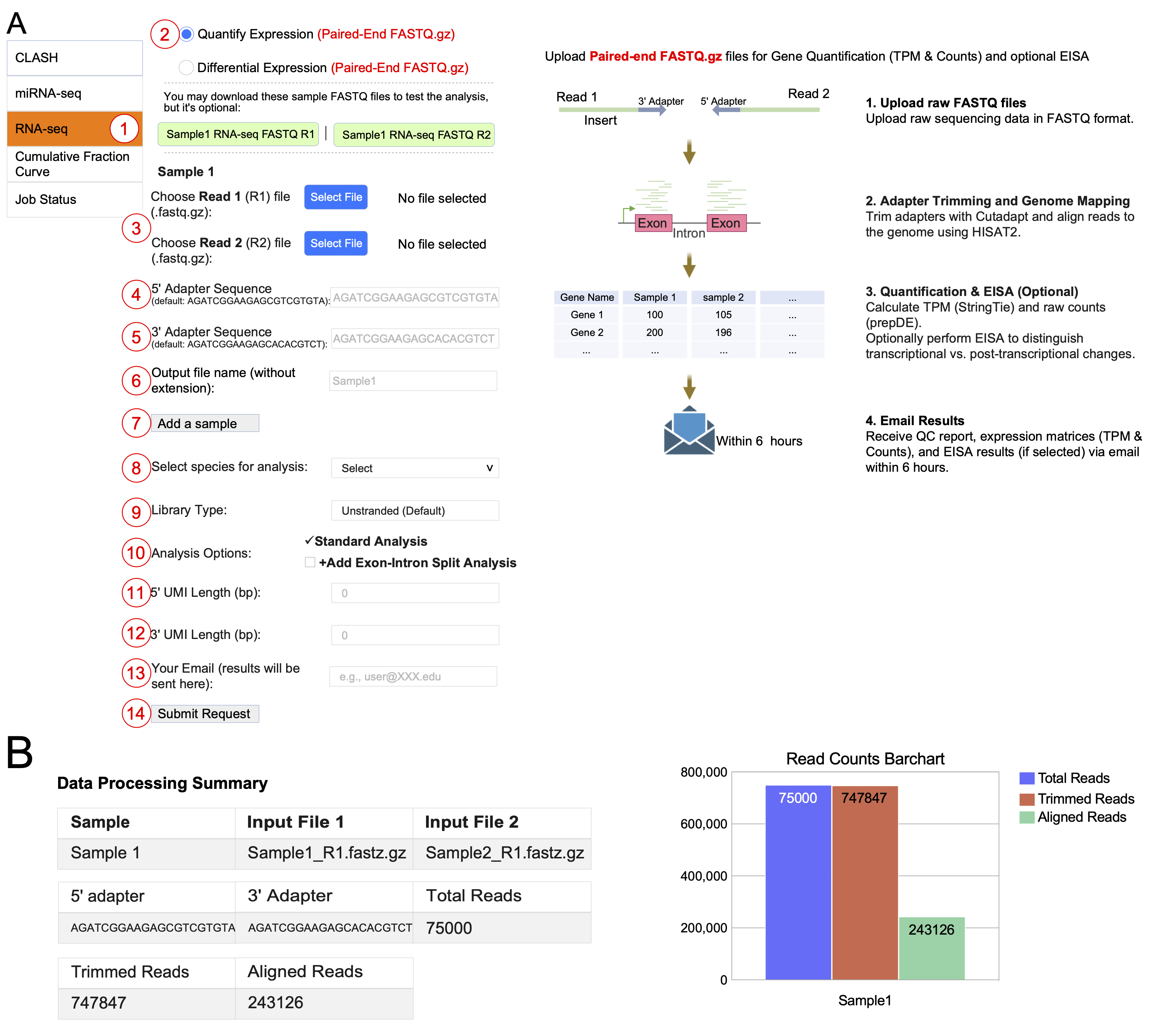
(A) Interface for RNA-seq gene expression quantification. Users 1 select the RNA-seq module, 2 choose paired-end FASTQ input, 3 upload Read 1 and Read 2 files, 4-5 enter adapter sequences, 6 specify output filename, 7 add more samples if needed, 8 select species, 9 specify the library type (unstranded or stranded), 10 configure analysis options (standard analysis is performed by default, with an option to add Exon-Intron Split Analysis), 11-12 define the length of 5′ and 3′ Unique Molecular Identifiers (UMIs), 13 provide an email address, and 14 submit the request. The backend bioinformatic pipeline to process paired-end FASTQ data is shown on the right.
(B) Example processing output showing adapter sequences, read counts across each step, and a bar chart summarizing total, trimmed, and aligned reads.
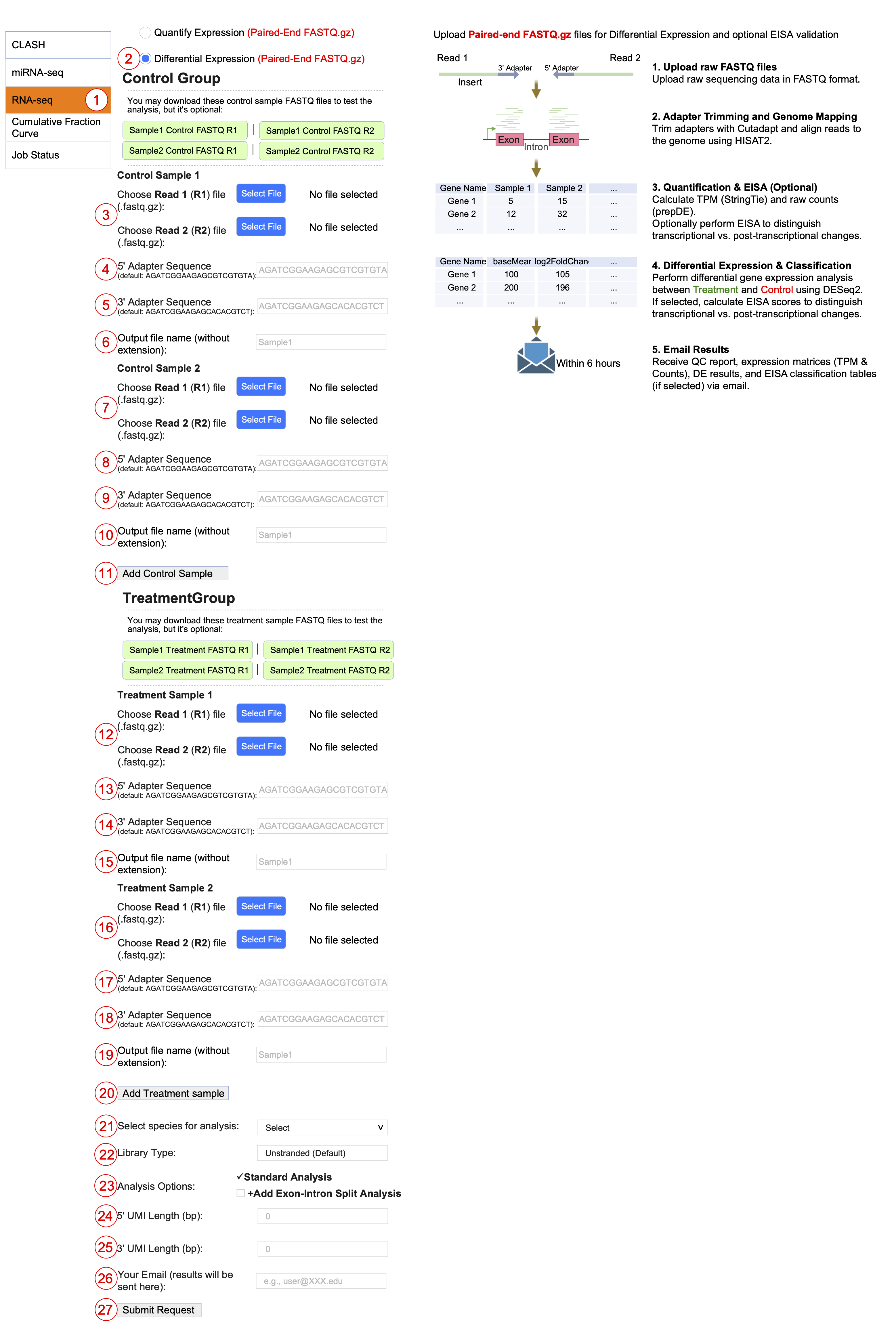
Interface for differential gene expression analysis. Users 1 select the RNA-seq module, 2 choose the differential expression option, 3-10 upload at least two control group paired-end FASTQ files with the option to add additional samples 11, 12–20 upload two or more treatment group files, specify adapter sequences and output filenames, 21 select species, 22 specify the library type (unstranded or stranded), 23 configure analysis options (standard differential expression is performed by default, with an option to add Exon-Intron Split Analysis), 24-25 define the length of 5′ and 3′ Unique Molecular Identifiers (UMIs), 26 provide an email address, and 27 submit the request. The backend pipeline that performs adapter trimming, genome mapping, count generation, and differential expression analysis is shown on the right.
Cumulative fraction curve analysis
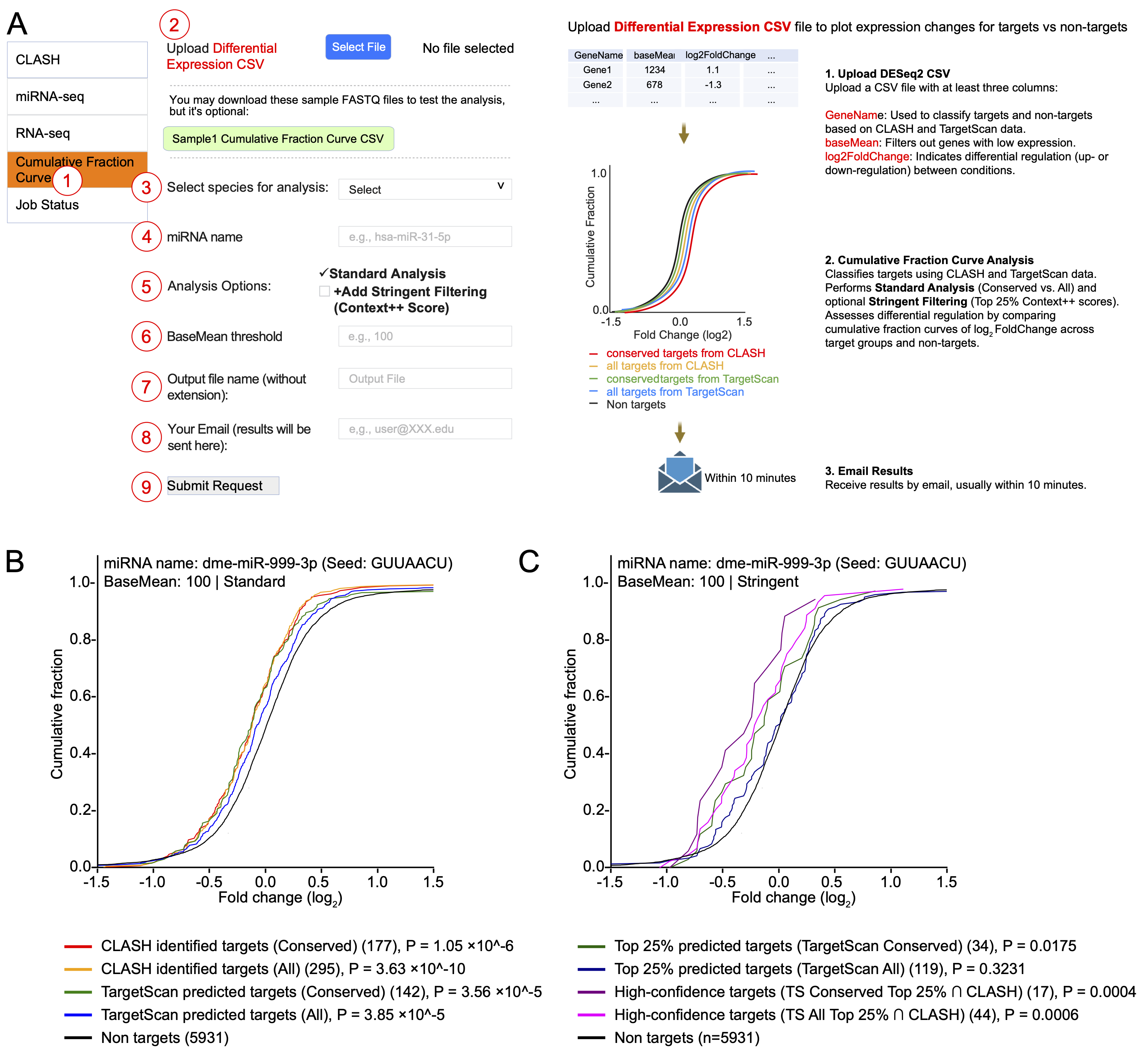
(A) Interface for generating cumulative fraction curves. Users 1 select the module, 2 upload a differential gene expression CSV file, 3 specify species, 4 enter miRNA name, 5 select analysis options (Standard Analysis and/or Stringent Filtering), 6 define optional miRNA count BaseMean threshold, 7 specify output filename, 8 provide email, and 9 submit the request. The backend bioinformatic pipeline to generate the plot is shown on the right.
(B) Example output of the Standard Analysis showing cumulative fraction curves for dme-miR-999-3p target classified by conservation status (Conserved vs. All) from CLASH and TargetScan datasets.
(C) Example output of the Stringent Filtering analysis for the same miRNA, displaying cumulative fraction curves for the top 25% of high-efficacy targets based on TargetScan Context++ scores and high-confidence overlaps with CLASH data. For both (B) and (C), Mann–Whitney U test P-values indicate the significance of expression shifts in target sets compared to non-targets.
Job status
The Job Status module allows users to monitor current job counts and query specific job statuses using a unique Job ID, enabling convenient verification of whether a job has completed, is in progress, or remains pending in the queue.